Building scalable networks

In this part of the lecture, we'll speak about how we can build scalable networks, that is networks that can handle a large (and growing) numbers of routers, routes, and prefixes. We'll do that considering both the control plane (routing) viewpoint and the data plane (forwarding) viewpoint.

First off, let me define what I mean by "large" network. Here, our goal should be to build networks that can have tens of thousands of routers, learning dozens of millions of routes, for up to 1.2 million prefixes. (Each prefix can have multiple paths associated to it, cf. BGP.) This is the realm of the Google, the Meta, the Amazon, the Deutsche Telekom, or the Microsoft of this world.

Being responsible for computating the forwarding state, the control plane will be affected by all these metrics: the size of the topology (the number of routers), how many routes are learned (that is, how many paths) and for how many prefixes.

In contrast, the data plane scalability will mostly depend on the number of prefixes it needs to cary.

As a reminder, the control plane is in charge of maintaining the routing tables (known as Routing Information Bases, or RIBs) which contain all the routes that the router has learned thus far; computing (and propagating) the best route for each destination prefix; and downloading the best routes for each destination prefix—that is, the forwarding state—into the forwarding table.

The forwarding table is often referred to as Forwarding Information Base (or FIB). A router uses its FIB to forward packets from one port to another. To sustain high forwarding speeds, the FIB is typically implemented in hardware, using SRAM. Doing so allows routers to forward at multiple Terabits per second.

We'll mainly see two scaling techniques in this lecture. The first one will help us improving how routes propagate within a network, considering both inter-domain routing (BGP) and intra-domain routing (OSPF). The second technique will help us reduce the number of entries in the forwarding tables by aggregating and filtering them away.

Let us start with how we can scale BGP route propagation in large networks.

As you know, BGP is the internet routing protocol we use today in the Internet. It's used between different Autonomous Systems, or ASes.

BGP is a path vector protocol: you have (AS) paths in the routing announcements, and each AS appends itself to the path before sending a route to the next AS.

BGP comes in two flavors. First, you have external BGP (or eBGP) sessions which run between routers located in different ASes. These sessions are used to learn/advertise routes from/to neighboring ASes.

Then you have internal BGP (iBGP), which runs between routers located in the same AS. iBGP sessions are used to propagate externally-learned (and internally-sourced) routing information within the network.

So for instance, iBGP allows all the routers in this US-based network to learn that they can reach this /16 prefix with this AS path using Seattle as the egress router.

Given a set of routes, BGP routers elect one best path for a prefix. BGP is often referred to as a single path protocol. The way to think about it is the following: let's say I'm a router, I know 10 routes for reaching one of Google prefixes, meaning I need to go from 10 to 1. What I will do is apply each of these steps in sequence until there is only one route left. Observe that there is a tie-breaking rule, meaning we are guaranteed to end up with a single route at the end of the process. So, you start with 10 routes, and then you will remove all the routes that do not have the highest local preference. Let's say you have 4 routes left. Then, out of these 4, you will remove all the ones that do not have the shortest AS path. Let's say now you only have 2, and then you continue to go down until you hit 1, which is then the best route. That's the route you propagate, not only externally but also internally, modulo policies (route-maps).

The different steps in the decision process can be divided in two sets: global and local steps. Global steps refer to globally-visible attributes (the preference, the AS path length, ...) which are directly attached to the BGP routes. At the end of the selection process, all the routers will have picked equivalent routes from the global steps viewpoint: all the routers will have a route with the same (highest) local pref and the same (shortest) AS path length. Note that you can have 2 routers that pick 2 different AS paths, but if one has a length of 3, the other one will also have a length of 3. The local steps refer to attributes that are local to a specific router and pertain mostly to hot potato routing. Hot potato routing is the idea that, when a network receives traffic, it should push it away as quickly as possible to minimize transit costs. There are two steps there: prefer eBGP routes over iBGP and prefer lower IGP metric to the egress router. If you are an egress router and you have some external session with others alongside with internal sessions, and your learn 2 routes, one external and one internal, you should prefer the external one if they are equivalent because it enables you to send the traffic away from the network instead of inside the network. Likewise, if you are a router inside the network, and you learn multiple internal routes that are equivalent again, then you would prefer one that comes from an egress that is closer to you than from an egress that is further away. So if I am here, a router in Zurich, and I learn a route from Basel and Geneva, and they are both perfectly equivalent, I mean much better practically to select the one in Basel because Basel is closer to Zurich and Geneva. So the traffic will take the shortest distance if it exits by Basel and Geneva from my perspective. Because these are local decisions, different routers would make different decisions based on this. A router in Lausanne, faced with the same decision, would obviously prefer to exit via Geneva rather than Basel.

Besides using the IGP to select routes, a BGP router would also use the IGP to figure out the physical next hop to use to reach an egress. For instance, if you are this Atlanta router over there and the next stop for this route is Seattle (which is not directly connected to you), then you need a way to figure out what is the physical next stop to use to reach Seattle. So this is where you would also use the IGP.

This process of figuring out the physical next hop for each BGP prefix is known as (recursive) next-hop resolution. Think of it as merging two routing tables. The first routing table, the BGP routing table, tells you that Seattle is the egress for that /16. The second routing table, the OSPF routing table, tells you that if you want to reach Seattle then you need to send the traffic to Chicago. Chicago is a directly-connected next stop.

This process happens on all the routers in the network. At the end, Atlanta will send the traffic to Chicago, which will send it to Kansas City, Salt Lake City, and Seattle, and then the traffic finally gets out.

This is an illustration of what I was saying just before about the hot potato routing step. If you are this router here in Houston and you learn two iBGP routes, one for which the egress is Seattle and the other one for which the egress is in New York. These routes have the same preference, the same local preference, 200, the same AS path length, 1, not the same AS paths, 20 and 40, but the length is the same, so they are equivalent from the BGP selection viewpoint.

Because the routes are perfectly equivalent, you will reach this step of the decision process. In this case, Houston happens to be closer to New York than Seattle, meaning that the traffic to this /16 will go to New York.

With hot potato routing, you tend to separate the network into zones. Assuming that external routes will come east and west (which is common for such a US-based network), somewhere in the middle, in the Midwest, routers will send left, while on the east side they send right. So there is kind of a frontier, somewhere around here, where you go left or right. You can think of it as with river. There are separation lines where one side of it you go to the Mediterranean and then the other side of it you go to the Atlantic.

So, inter-domain routing in a nutshell. In eBGP, you learn and advertise routes from and to your neighboring AS. iBGP is used to disseminate internal and external routes within the AS, and the IGP, or OSPF, shortest path routing, helps you compute the shortest path routes within the AS and to identify the closest egress point.

We are now ready to start talking about scalability.

One thing we have always told you in your intro lecture is that iBGP routers do not redistribute iBGP routes to one another. That means if I'm an iBGP router, and I learn a route from another iBGP router, I don't redistribute that route to any other iBGP router. With this rule in place, the only way to guarantee full propagation is to create a complete graph of iBGP sessions amongst all routers. That is, we need a full mesh of BGP sessions.

That's a lot of iBGP sessions: n(n-1)/2, where n is the number of iBGP routers. With 100 routers, you have to configure 5k sessions, and with 1000 routers, which is again the ballpark number we are targeting, we end up with half a million iBGP sessions configured. There is no way you can do that manually.

Even if you automate this though, it's still very annoying to have each router maintaining half a million iBGP sessions. First, it's a lot of TCP connections to maintain. Second, you will often end up with your routers learning too many BGP routes. Then, whenever a router updates its best route, it would have to send that update to half a million neighbors (which consumes CPU and bandwidth). The killer argument though is that, whenever you add or remove a router in your network, you need to touch every single other router in your network to add or remove the corresponding session. This is extremely annoying in terms of network operations.

One solution, which is heavily used in practice, is known as BGP route reflecction. As the name indicates, route reflection allows some iBGP routers to reflect routes that they learn over an iBGP session onto another iBGP session. Doing so allows to create a hierarchy of iBGP routers, with route reflectors sitting above client routers.

One of the classical insights of computer science, which says that whenever you want more scalability, you should introduce a hierarchical structure, very much applies here.

BGP route reflectors establish "normal" iBGP sessions. The only thing that changes is that, in the configuration, some sessions are indicated as being client sessions, while others are indicated as being peer sessions. Route reflectors establish peer sessions amongst themselves (i.e. with other route reflectors) and client sessions otherwise.

This is a first example of route reflection topology (on the right). Each of the clients (RA and RB) only maintains one single session with their route reflectors (RR1 and RR2) which in turn maintain a single peer session in-between them.

If a route reflector learns a route from a peer (another route reflector), it will relay it to its clients (customers), but not to its other peers. While if a route reflector learns a route from a client, it will relay it to everyone. You might recognize here a connection with the classical propagation rules you know in eBGP based on customer, peer, and provider sessions. (The two logics relate indeed.)

Let's look at an another example. Similarly to the example above, you can see that there are two route reflectors: RR1 and RR2 connected by a peer session. RA is the client of RR1, while RB is the client of both RR1 and RR2. (For redundancy purposes, it's good practice to ensure that each client router is connected to at least two distinct route reflectors.)

As I said, to whom a route reflector reflects depends on the session types on which the best route is learned. So if RR1 learns a route from its client, RA, it will reflect it to everyone, including RR2. Upon receiving the route, and assuming its the best route, RR2 will also reflect the route to everyone (except the session onto which it has learned it), meaning RB will receive two copies of the route, one via RR1, the other one via RR2.

This slide considers the case where RR2 learns a prefix over an eBGP session that it reflects to everyone, peer and client. RR1 will then reflect it back to its own client, RA, because it comes from a peer. Observe that, unlike RB, RA only receives one copy of the route, since it has only one route reflector.

Route reflection allows to scale, but comes at the cost of route diversity. In a full mesh, each router is learning all the globally-preferred routes known for a prefix. In contrast, with route reflection, each router will only learn the best route advertised by its route reflector(s). Often this means going from having routers learning dozens of paths towards the same prefix (one per egress router learning a globally-preferred route) to two or three.

Besides routers might end up using different routes when in a route reflection topology than when they are using a full mesh. In other words, there can be be suboptimal routing. This is because the route reflector is making its own decision based on its own local attributes. The decision step pertaining to the IGP distance I was referring to before is now done from the route reflector's viewpoint, so the route reflector will make local decisions that are then reflected towards the clients. In other words, clients are not (necessarily) making their own local decision anymore.

Let me give you an example of that. We have a simple network with RA, RB, and RC that act as egresses for the network. RA learns one external route, r1, RB learns r2 and r3, and then RC learns r4. These routes are for the same prefix, and they are equally-preferred: they have the same local pref, same AS path length, etc.

In this case, RA would select R1, RB would select r2 (because of the tie-breaking step, assuming r2 comes on the session with the smallest peer address), and RC would select r4. So if we are looking at an iBGP full mesh, RD would learn r1, r2, and r4. RD would then prefer r1 based on the IGP distance to reach each of the egress (2 is less than 5 or 6).

Now, let's make the router in the middle, RE, a route reflector. We remove the full mesh, and we just add client sessions between RE and RA, RB, RC, and RD. As before, RA, RD, and RC, we select r1, r2, and r4, that doesn't change. They advertise that now to their route reflector, which is RE.

And now RE will select, from its own viewpoint, what is the best route there. From RE's viewpoint, to reach A is a cost of six; to reach B is a cost of one; and to reach C is a cost of two. So RE is taking a different decision than RD and it will pick r2 which it then reflects it to all its client, including RD in this case, which will only learn one single route instead of three, and this route will be r2, with RB as the egress. This is a very clear case of suboptimal routing. It's correct, the traffic is not dropped, and there is no loop here or black holes. But we are now using a longer path than what we would have taken in a full mesh. That's the price to pay for route reflection.

Of course, how suboptimal the routing becomes depends on the position of the route reflectors. And you can phrase that as an optimization problem, but we won't go into details of that optimization problem in this lecture.

With route reflection, things can get worse than "just" suboptimal routing though. Route reflection can indeed lead to both routing and forwarding anomalies. Forwarding anomalies are of two types: forwarding loops and black holes. Routing anomalies include problems such as permanent oscillations and multiple stable states. Route reflection, when done wrong, can cause both anomalies.

Let me first give you an example inducing forwarding loops. Granted, I'm creating weird route reflection topologies in order to create these anomalies, but these are perfectly legit.

So now I'm considering the same example as before, with two route reflectors, A and B, and then I have two clients, C and D. But as you can see, I have swapped over the client session. So now we kind of have like the route reflection topology is not in sync anymore with the physical topology. So instead of having RC be a client of RA, RC is a client of B, and RD is a client of A. So your client would be at the opposite corner.

And for A and RD, they appear as before. So as you can see, A learns a route for one, and then B learns another route for two.

Again, the same prefixes that are all equivalent as before. So RA and RD will reflect that to their clients, C and D, meaning what? Meaning that C we learn R2 and D we learn R1. See what I mean?

So what is the shortest path between RC and R2? Well, it's RD, RRE. What is the shortest path between RD and R1? Well, it's RC, RRA. So as you can see now, we have a forwarding loop between these two routers that has been formed.

This is a permanent forwarding loop, so the traffic will forever be dropped in between these two routers, unless, of course, you realize it, and then you change the configuration. But this is a classical example of the problem. Again, it can be subtle.

This problem will only manifest when you have exactly these two. A route on A and B that are equivalent, for which then the problem happens. But if you had only a route of A or only a route of B, you would not have the forwarding anomaly appear.

So again, I just want to tell you that verifying a network is not something that you really can do at scale. So traffic is now trapped in a forwarding loop. So that's an example of forwarding anomalies.

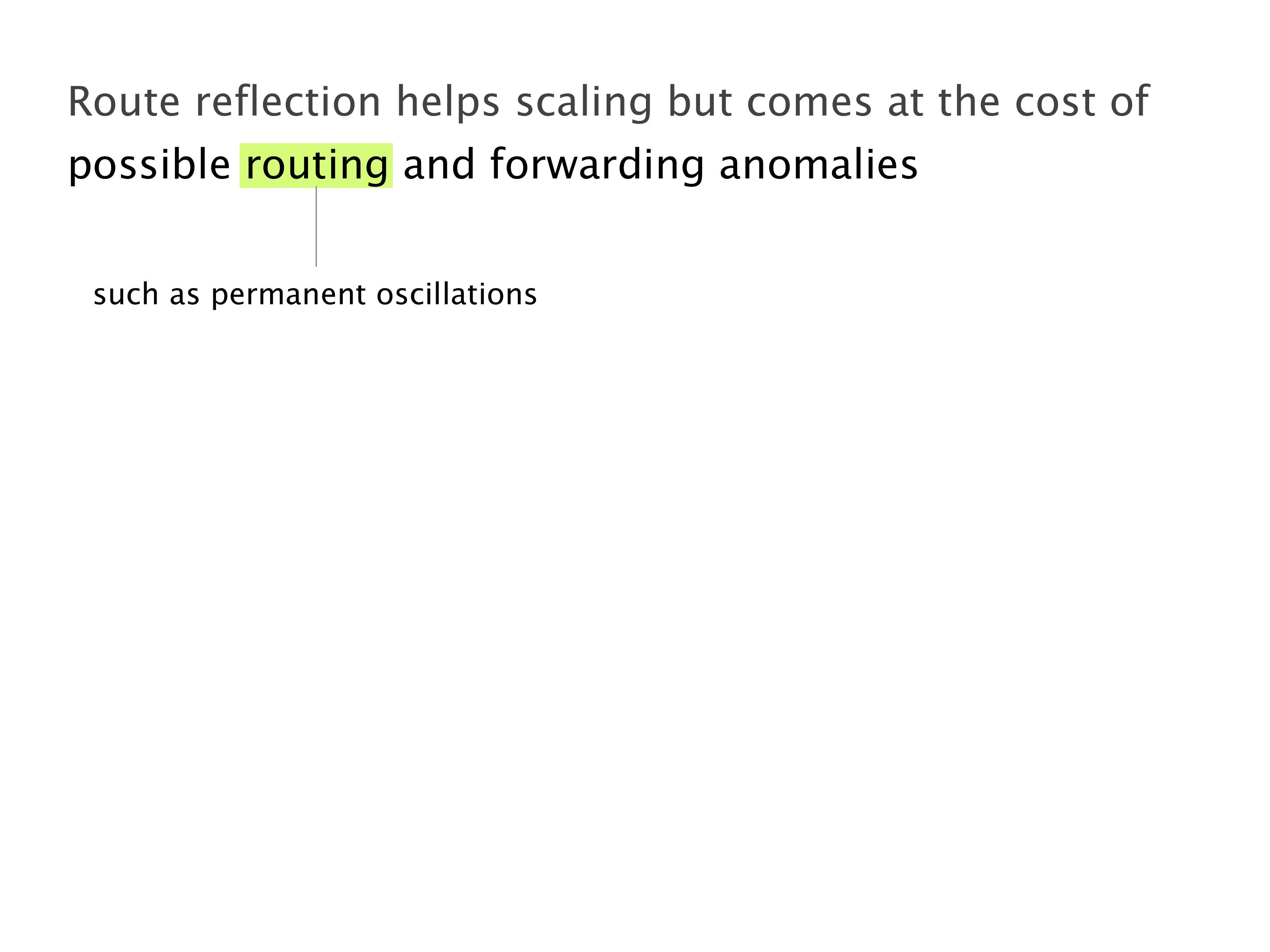
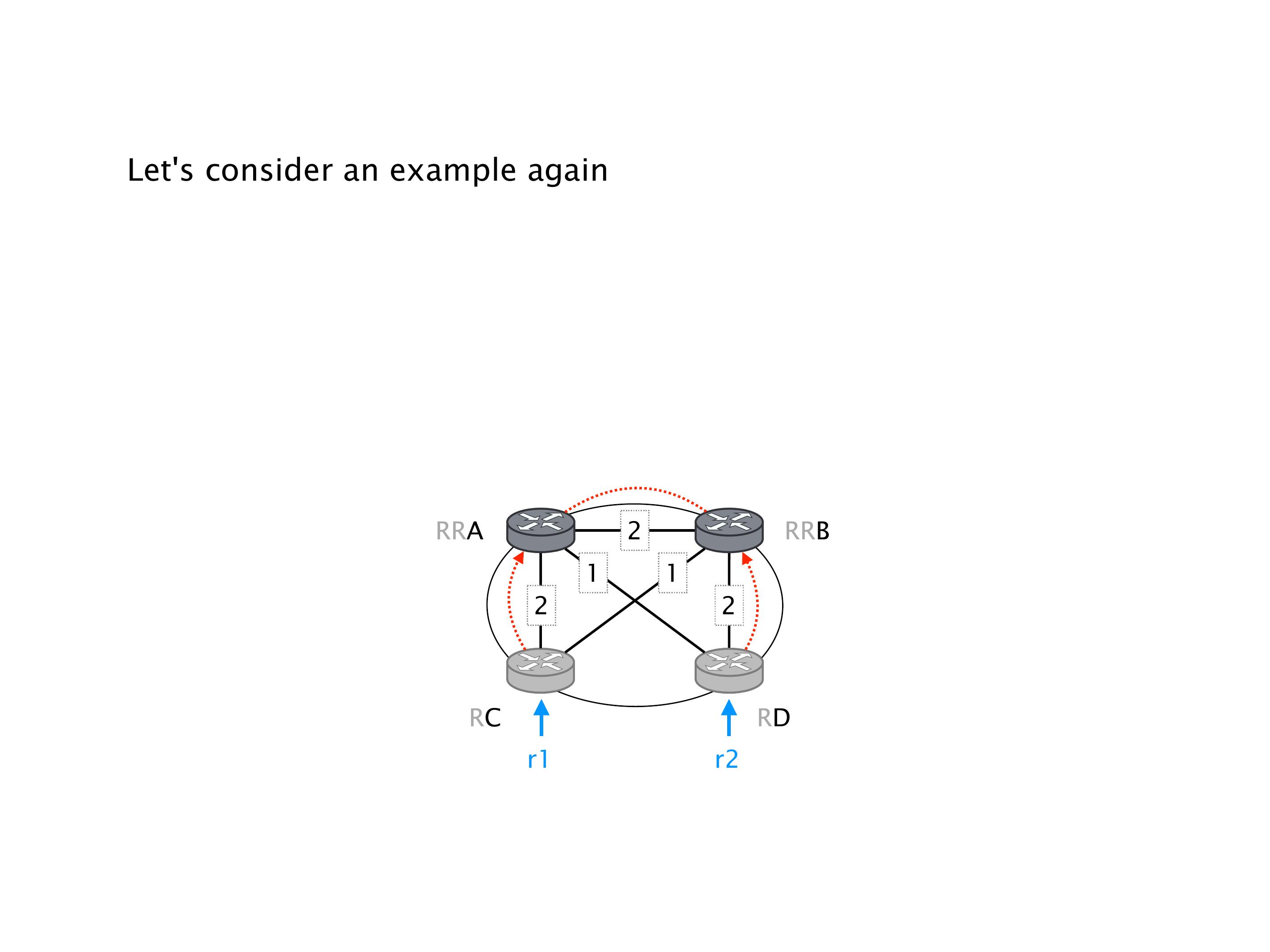
Another example of anomalies at scale are permanent oscillations. So again, this is a little bit of a crazy network, but I'll just give you one example where it happens.

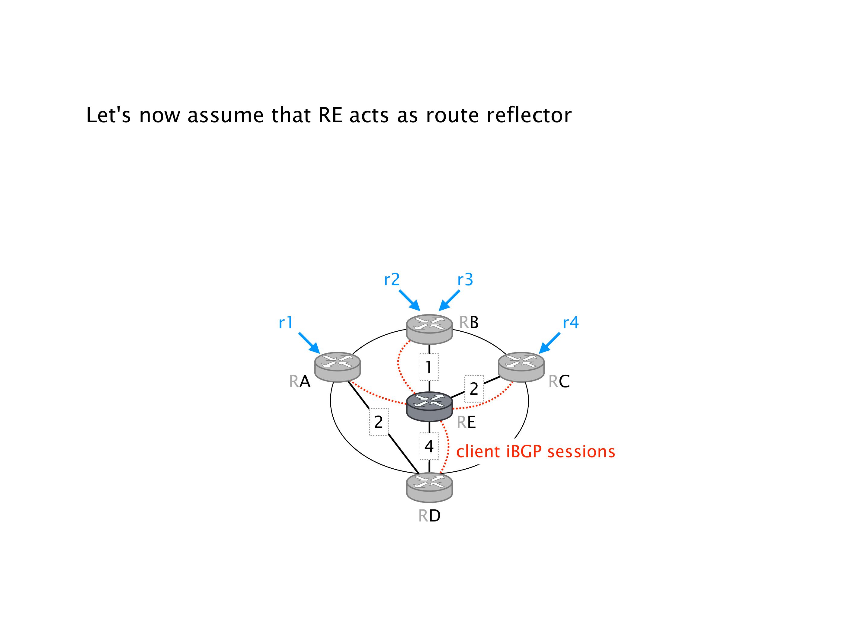
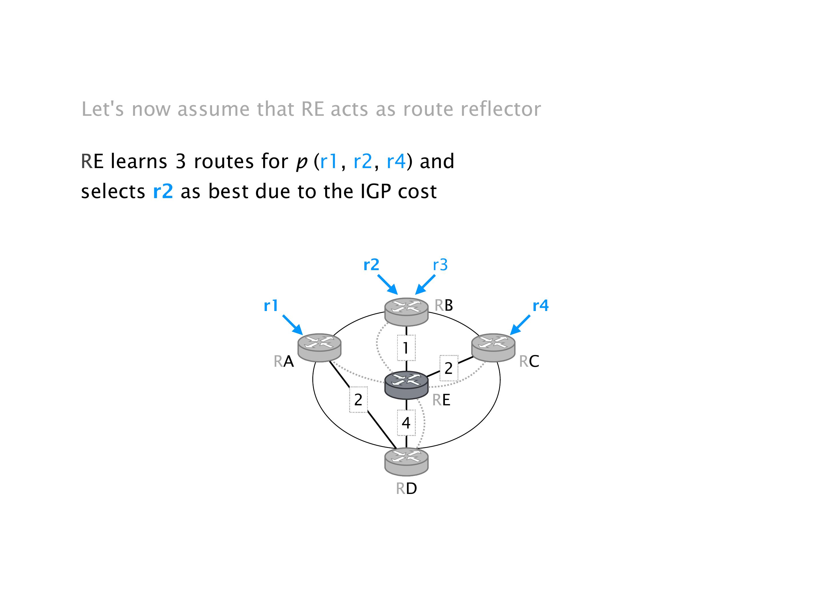
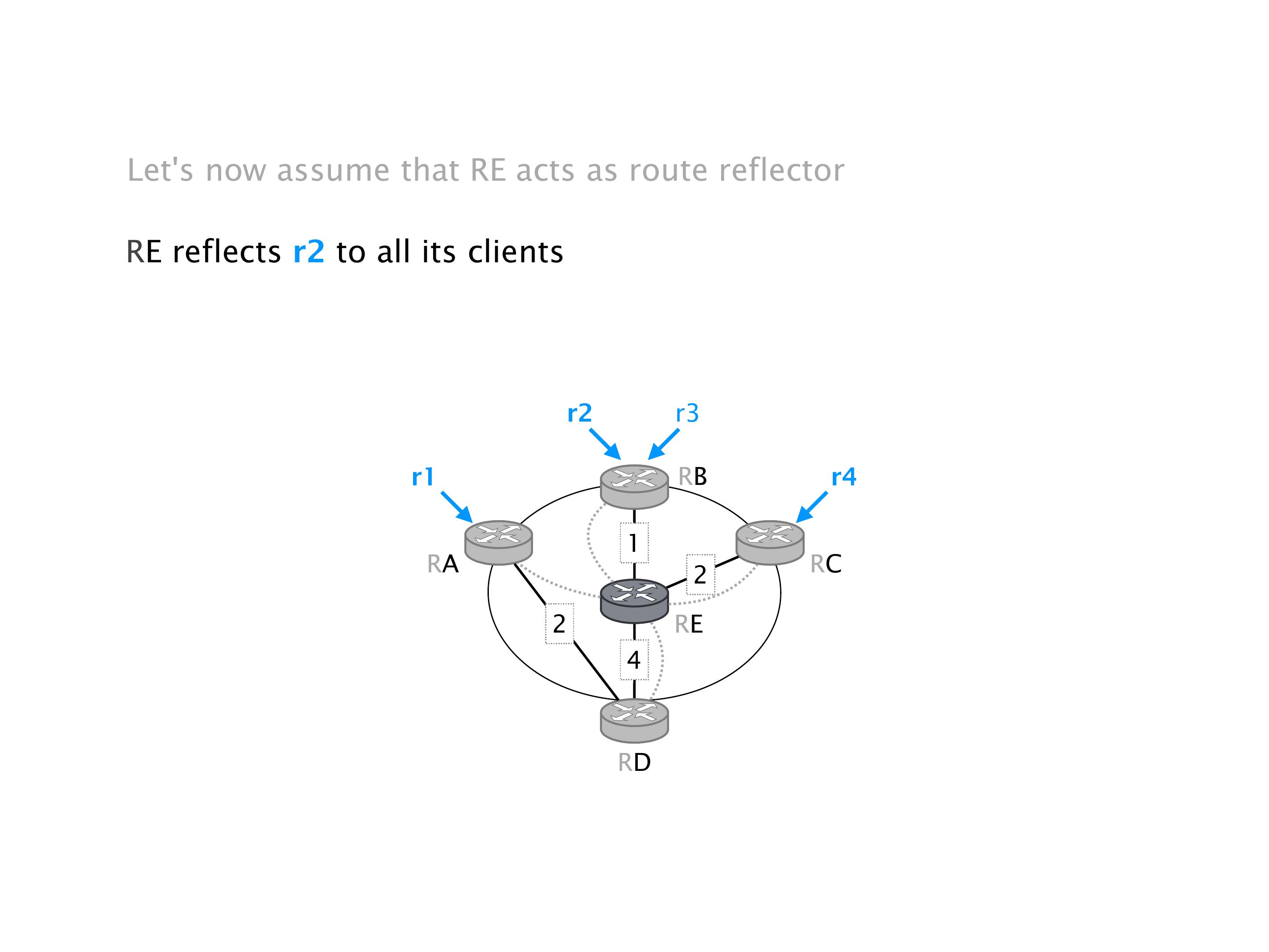
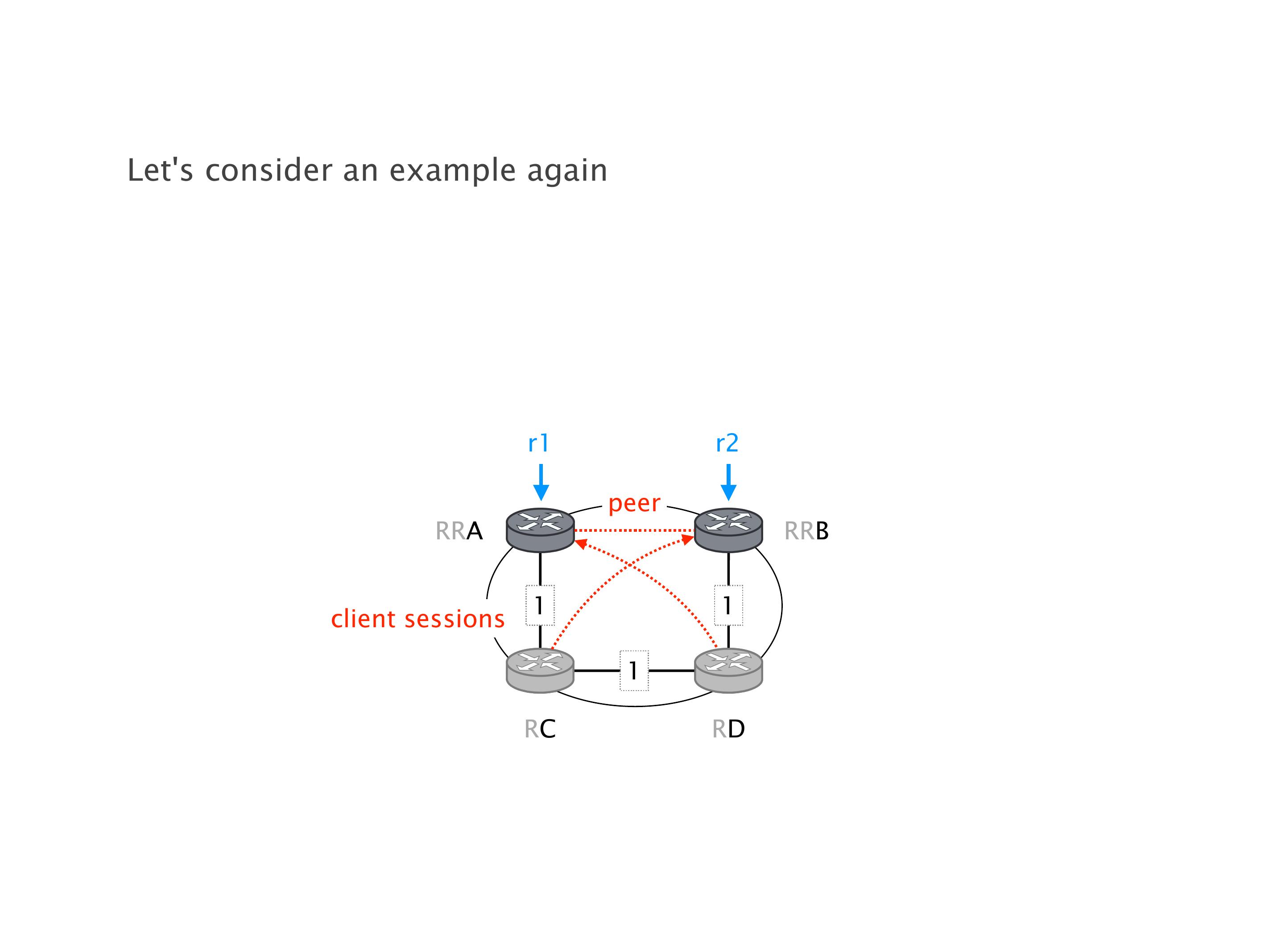
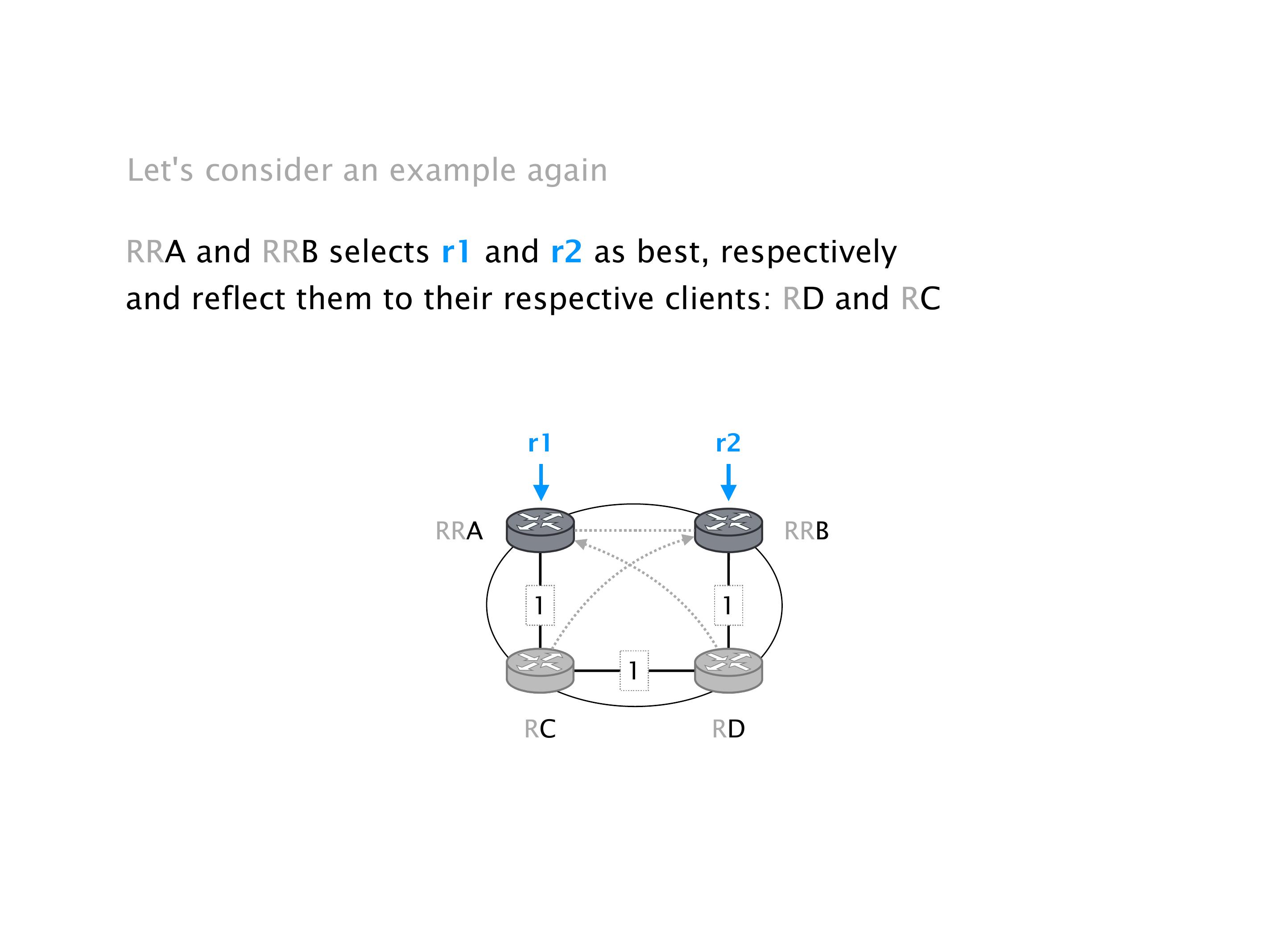
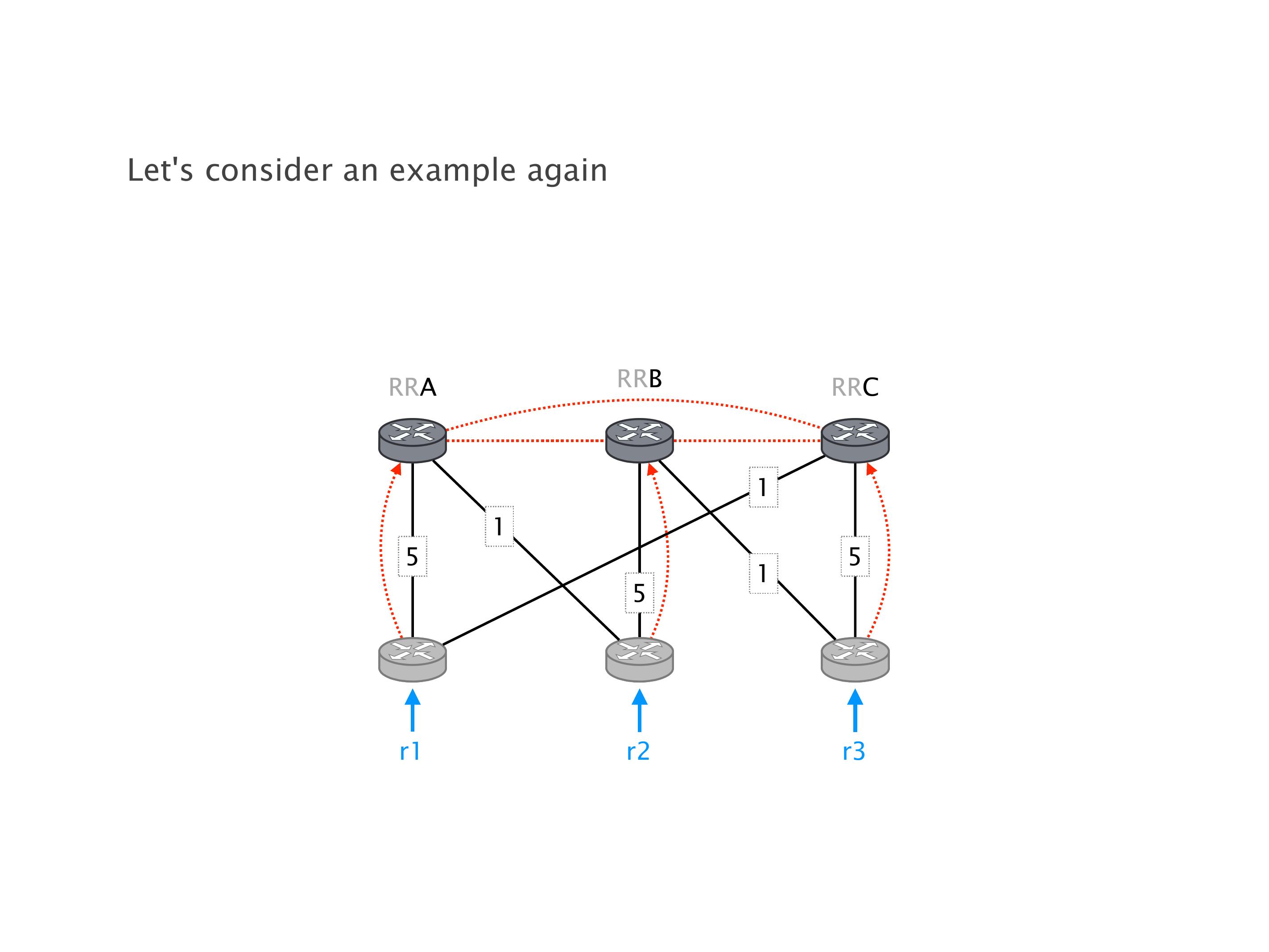
Here you have a topology with three vertices around the bottom. One there is R1, one there is R2, and one there is R3. And then you have three route reflectors. The route reflectors are totally fine. There is a full mesh of peer sessions between tier ones.

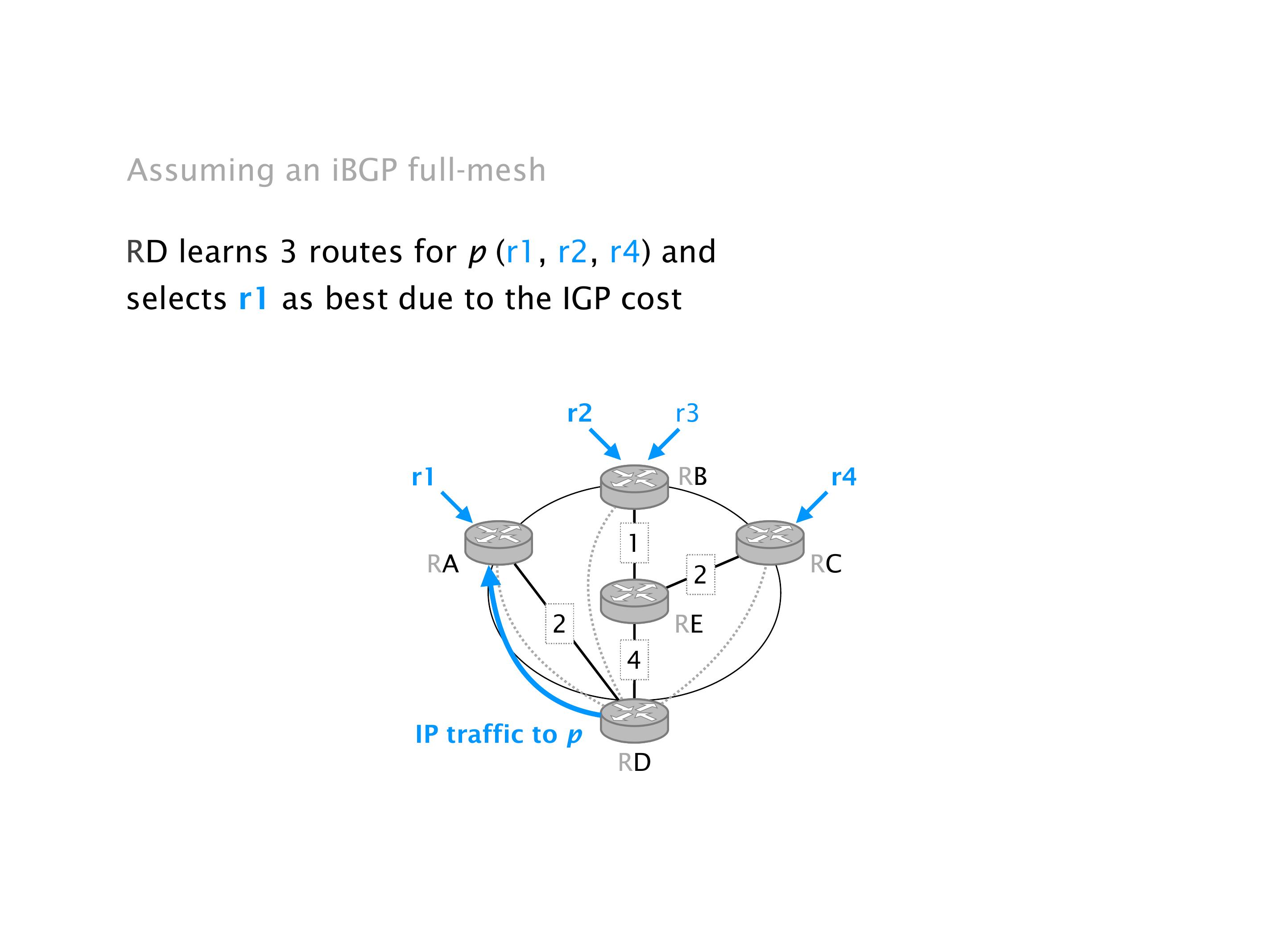
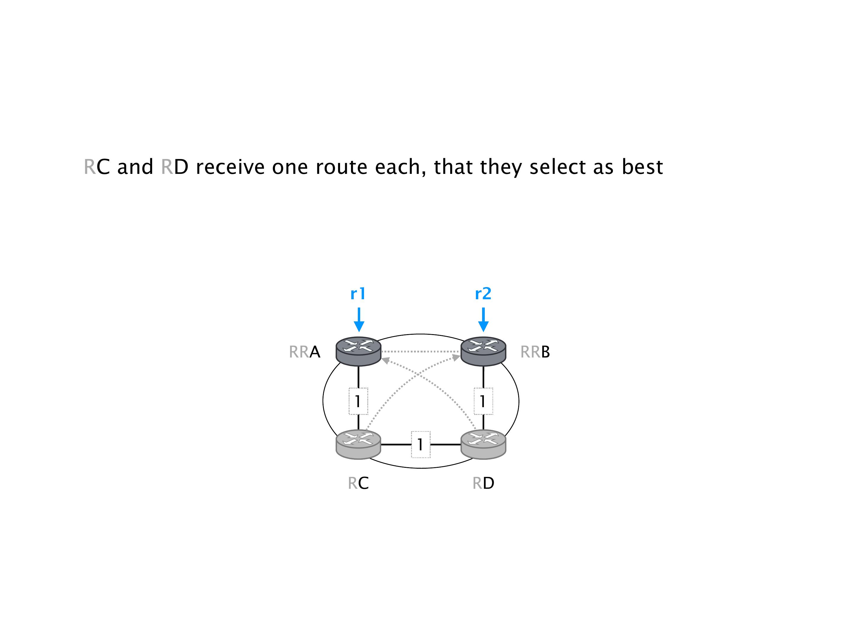
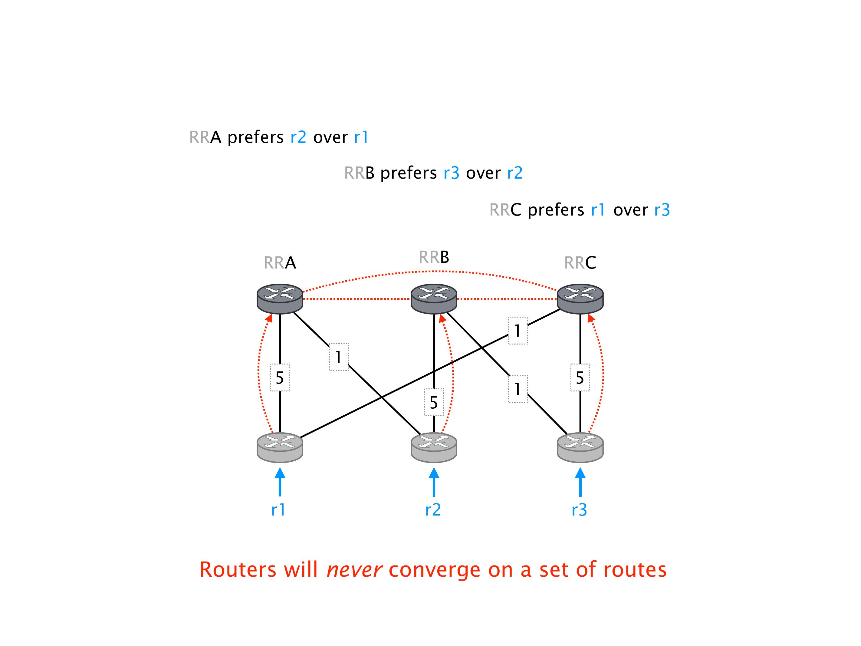
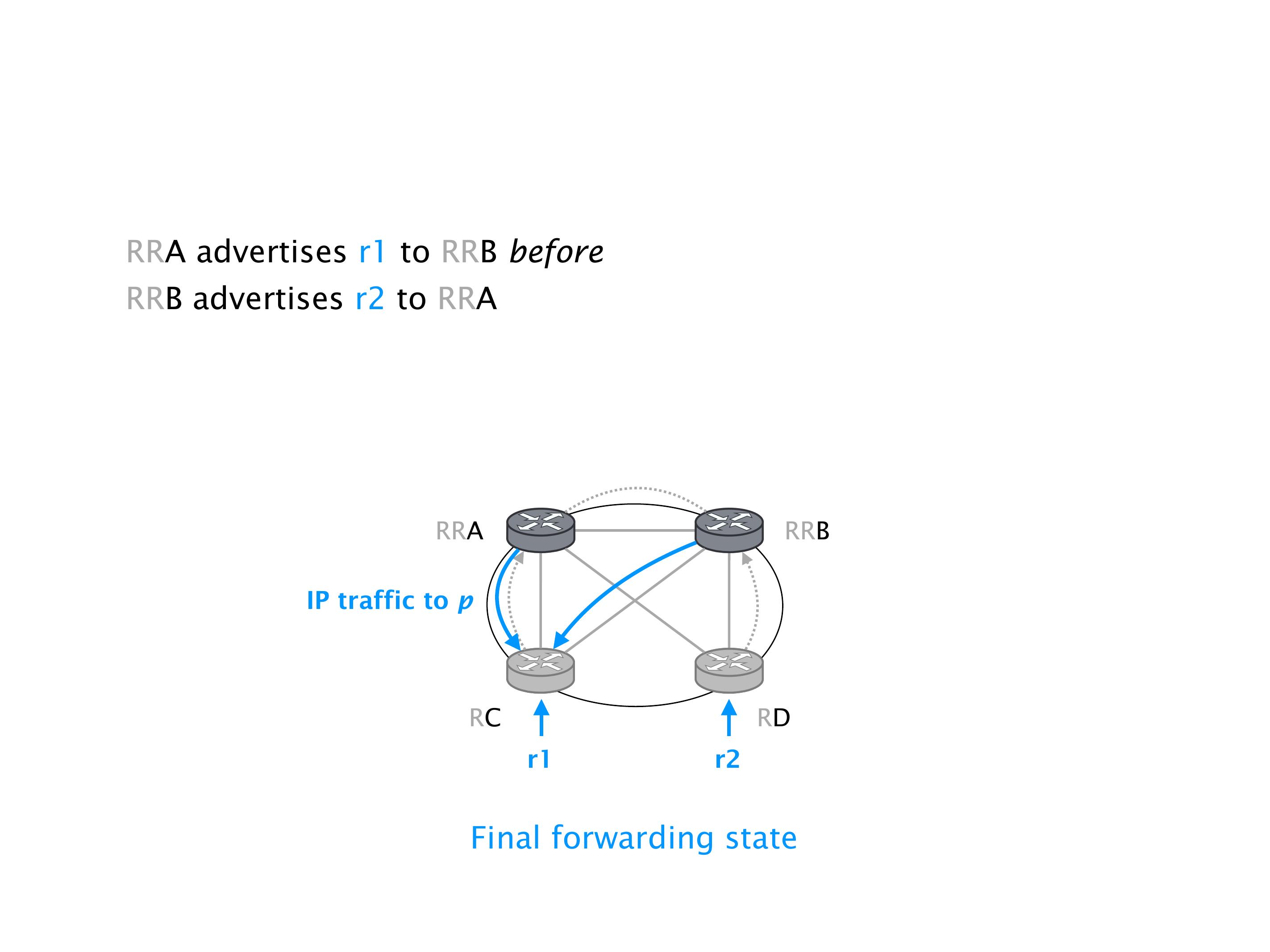
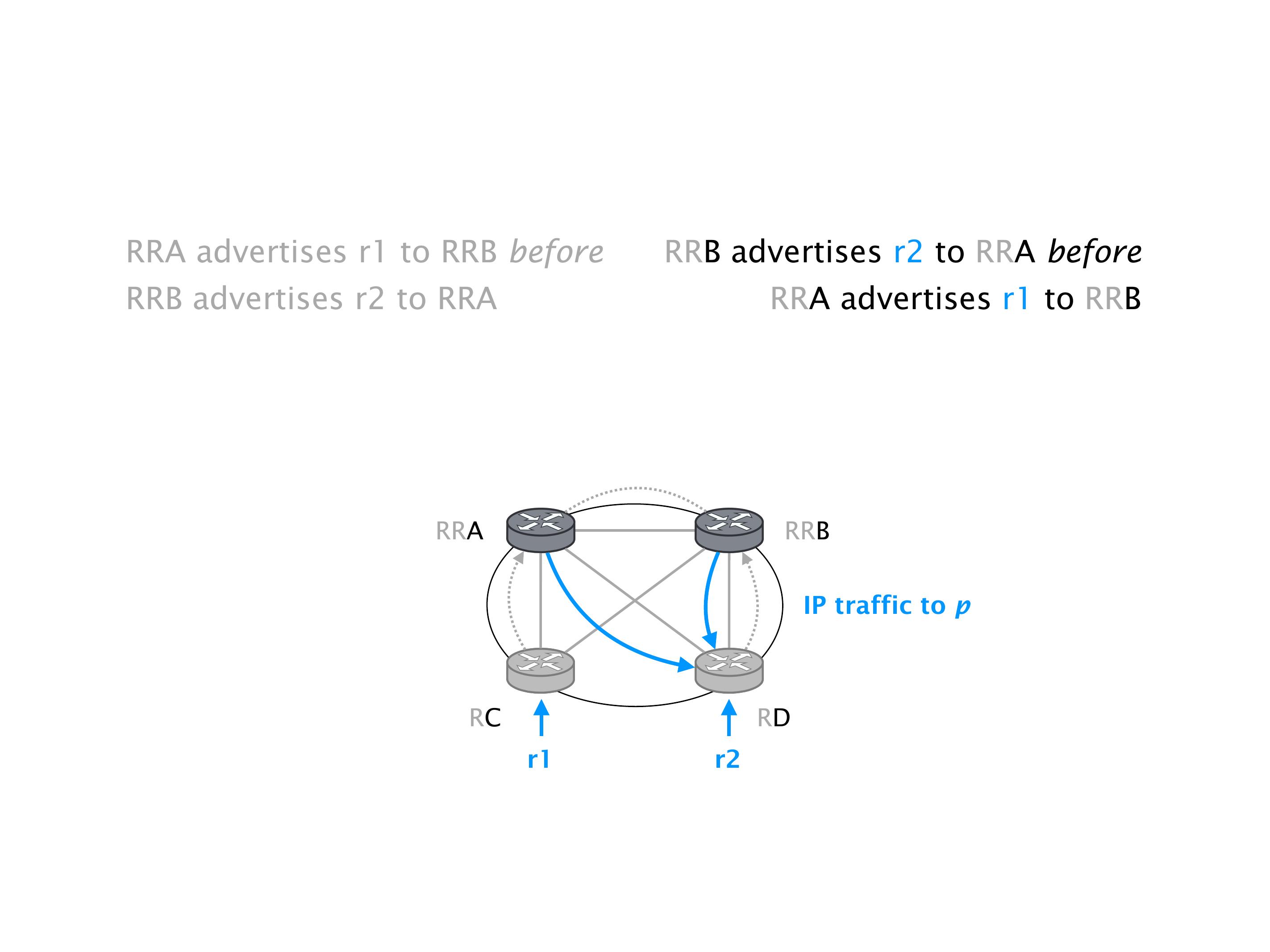
Again, same thing. And then this router is the client of A, this router of B, and then this router is the client of C. But then this is where the weirdness happens. If you look at the preference of A in terms of IGP cost, A is closer to this router than to that router's client. So A prefers R2 over R1.

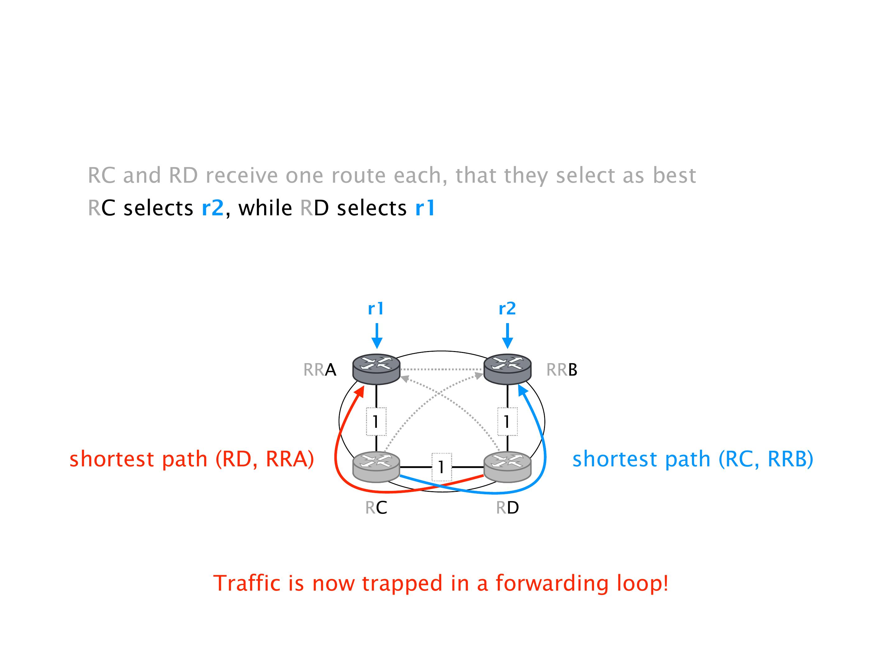
B is closer to R3 than it is to R2. So B prefers R3 over R2. And then, finally, C prefers R1 over R3. So again, you can see now we have a cyclical relationship here, where each router prefers a router on the right, like a torus kind of thing, where C goes back to A.

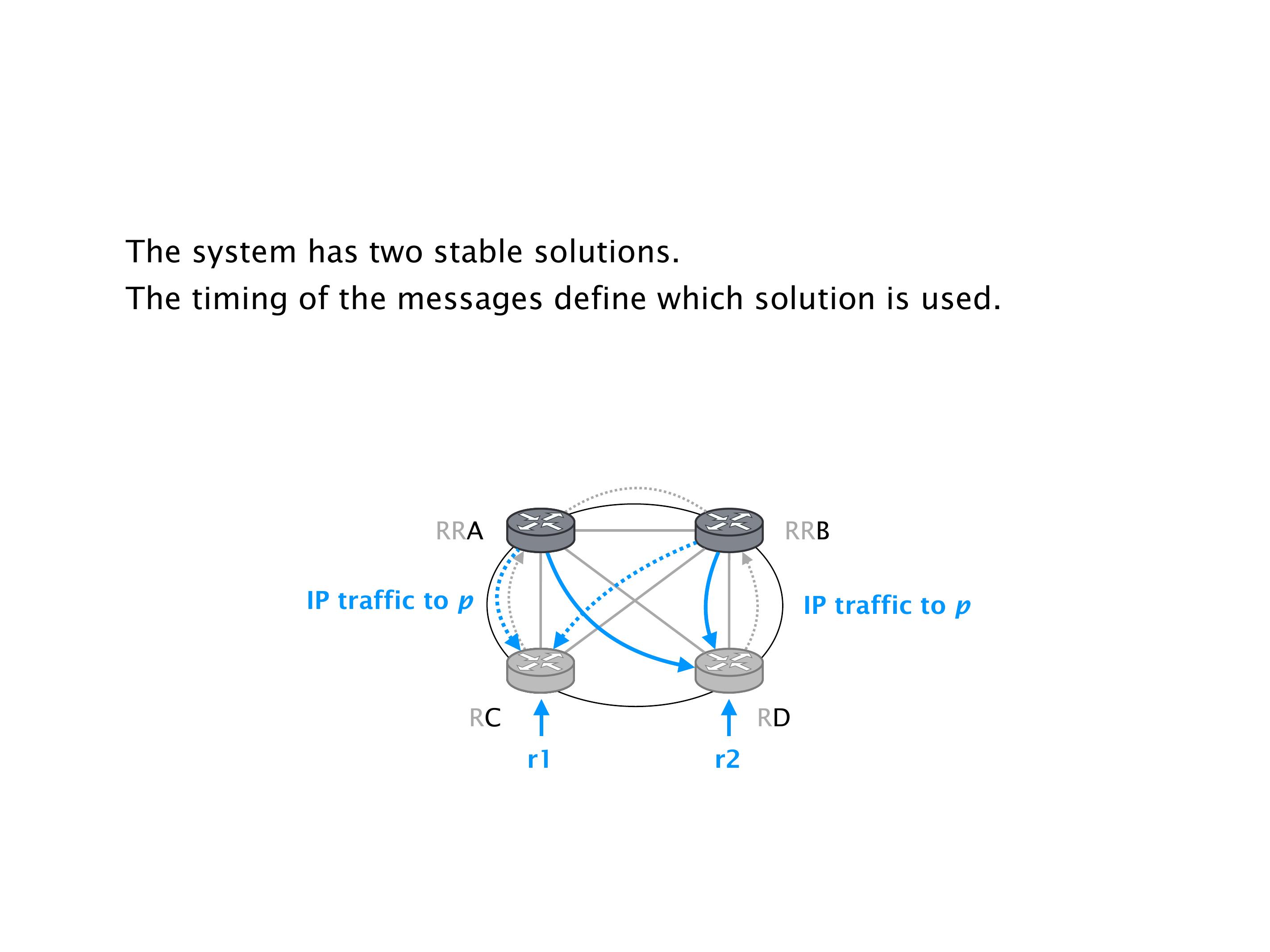
Here, you would do that in the exercises. But this network will never converge. So if you configure this network, again, you can, nothing prevents you from spinning up a virtual network, and then configuring the network like that, you will see that the routers will forever exchange routes. They will never converge.

It doesn't necessarily mean that the traffic will be lost. It just means that sometimes RA will go here, and we send the traffic to R2, sometimes we send it to R1, etc. So the traffic will keep shifting, not necessarily being dropped. You can combine oscillation with the forwarding loops, in which case the oscillation creates the forwarding loops. These are the most extreme cases. But that wouldn't be the case over there.

Still, it's very annoying for traffic to oscillate. Again, if you think about what TCP does, TCP is trying to estimate the delay, the RTT, the round-trip time between the source and the destination. And it needs a little bit of time for that. It needs some packets in order to measure this. So if the paths keep changing, then the estimates of TCP are kind of pointless because the two paths can have drastically different RTT in practice, meaning that the behavior of TCP will continue to shift as well. So we have poor performance. TCP really doesn't like jitter, meaning variance in the RTT. This is why it's bad. And also, you have your router forever doing work, which is useless.

The last problem I'd like to talk about is non-determinism. What I mean by that is that there are multiple solutions that can be computed, multiple stable solutions, and you do not know which one will be picked. This is very annoying from an operational viewpoint, because you cannot reason about what your network will do in advance.

In this example we have two route reflectors, RRA and RRB, and then we have these two clients, RC and RB. RC advertises r1, and then RB advertises r2. What you have to see is that RRA prefers r2 over r1, because it has a cost of one to each RD and a cost of two to each RC. RRB is exactly the opposite. It prefers RC over RD.

So what happens? Well, let's say, this router over there, it's a bit faster than this router over here to announce the route to the route reflectors. So RRA wil learn r1 first, and then reflect it to RRB. In this case RRB is happy: it has learned its best route. This means that, later on, when RD finally advertises r2 to RB, RB doesn't reflect it because this is not its best route. In this situation, RA looses.

Of course, you can have the symmetrical case, in which RD is the first one to advertise r2. In this case, the network stabilizes in another configuration where RA is the happy one. This non-determinism is an issue. Since you do not know if the traffic will go left or right, it's hard to do things like capacity planning, for instance.

Note that this is not an oscillation, the network does stabilize, but you do not know in advance into which state.

Unfortunately, deciding whether a given route reflection is correct or not is NP-hard, meaning there cannot exist an efficient algorithm to answer this question in the general case (unless P equals NP, and let's not go there).

So what do you do though? It's not like the internet is falling apart all the time because of this. So there must be something afoot there that allows this to work.

Luckily, sufficient (not necessary) conditions for correctness are known. This means that if you configure your network following these guidelines, you will be guaranteed that there will be no problem. If you don't follow these guidelines, then you may or may not have a problem.

The first condition is to ensure that route reflectors prefer the routes coming from their clients over the routes coming from their peers. In a lot of the examples I was showing you, this was not the case. You had one route reflector that was preferring the routes of the client over the routes from other route reflectors. That's bad, because then you can start to combine this into a preference circles.

The second condition is to ensure that "BGP messages follow the data path". That is, that every shortest path between any two routers should be a valid “signaling path”. If we look back at the example of slide 57, that was clearly not the case. There we could see that the shortest path between RC and RRA (resp. between RD and RRB) was not a valid signaling path (there was no corresponding BGP session on it). This conditions allows to guarantee the absence of deflection. Deflection happens when different BGP routers along a forwarding path choose different egresses. Again, in slide 57, we had RC picking RRB as egress, and RD picking RRA as egress, and both of them lying alongside the shortest path of one another towards the selected egress.

Slide 69 is another example of a network which violates the second condition every shortest path between any two routers should be a valid signaling path, which creates a deflection.

In this network, there is only one route reflector (RR1) which connects to two clients (C1 and C2). Both RR1 and C2 learn an equally-preferred route for a prefix p (r1 and r2, respectively).

As you can see, the shortest path between C1 and C2 is the direct link (C1, C2). This shortest path is not a valid BGP signaling path: BGP routes do not flow alongside it. Here, there is only one valid signaling path between C2 and C1: C2, RR1, C1.

Because of this a deflection arises. Here, RR1 chooses r1 as best route, and propagates it to C1 and C2. C1 therefore selects r1 as best. C2 though learns both routes: r1 from RR1, and r2 from its eBGP peer. Out of the two, C2 prefers the external route (eBGP routes are preferred over iBGP routes).

Now, observe that the shortest path between C1 and RR1 goes via C2. This means that when C1 sends traffic to p (which it believes will exist via RR1), it hits C2 which then forward the traffic out instead of towards RR1.

While this deflection looks innocent at first, it isn't. Amongst others, it can lead to forwarding loops across different ASes since traffic does not follow the AS-PATH anymore. (If you are interested, you can check Figure 16 in this paper for an example.)

In Slide 70, we have turned C2 into a route reflector (and renamed accordingly to RR2) and connected it to C1 as well. Now, the condition that every shortest path should be a valid signaling path is respected since there is an iBGP session and BGP messages "flowing" alongside (RR2, C1). This network is not subject to deflections. Here, C1 will select r2 as egress and traffic will indeed leave via RR2.

In most cases, you'll see a single level of route reflection. But just for you to know, you can actually create multiple levels of route reflection, should you want to do that. So you can have a route reflector that has client route reflectors that themselves have clients. You can have as many layers as you want. So you can stack these route reflection layers on top of one another. Finally, you can configure route reflector with what is known as a cluster ID, which as the name indicates allows to group route reflectors into clusters.

Let us switch gear now and speak about and how we scale link-state-like IGPs.

In link-state routing, as you know, what happens is that the routers build a map of the network graph by flooding link-state advertisements. Each router maintains its incident links and costs and then floods that throughout the entire network. Think of it as a tiny piece of a puzzle: each router knows its local view and then sends that to everyone else. Everybody puts the pieces together, builds a graph, and then runs Dijkstra on it.

What's distributed in OSPF is not the computation. Each router locally run Dijkstra on the reconstituted graph. Instead, what is distributed in OSPF is the flooding of the graph. In BGP (and, more generally, distance-vector protocols), the computation of the routes themselves are distributed. So it's a very different family of protocol, they work (very) differently.

So what are the scalability challenges behind link-state routing? Well, the larger the topology, the more work it will take for the routers to flood. Likewise, the large the topology, the larger the graph to store. And then, of course, the larger the topology the more time it takes run Dijkstra on it. So, you need more bandwidth for the flooding, more memory to store the graph, and then you need more compute time to run Dijkstra.

How do we improve scalability? Well, the first part is to reduce as much as possible the overhead of the algorithm. That means trying to reduce the amount of computation you need to do and reduce the frequency at which you do these computations.

The second step is to introduce a hierarchy. Similarly to what we have done with route reflection.

Let's talk quickly about reducing the algorithm overhead.

The first thing is to make sure that you use optimized data structures. In your introduction lecture, you may have seen simple versions of Dijkstra that were running in $\mathcal{O}(n^2)$, where $n$ represents the number of vertices in the network. Using a heap, you can reduce the complexity to $\mathcal{O}((m+n) log(m))$, where $m$ represents the number of edges.

The second thing, when there is a change, you might not need to recompute the entire forwarding state (i.e. that is, recomputing the shortest path towards all other nodes). You might be able to reuse some portions of the existing shortest paths. In short, you can make the algorithm incremental.

The last technique is simply to run the algorithm less frequently by e.g. pacing the computation. You make the router wait a little bit before recomputing. This is very useful, for instance, when you have links flapping, that is, links that go down, up, down, up, etc. These are very typical failures. Since each router recomputes its shortest paths every time there is a change in the graph, the entire network is recomputing shortest paths with each link flap. Pacing can help here. Of course, if you are too aggressive with your pacing, then you run into the risk of having your routers not immediately reacting in case of a real failure. As usual, this comes with limitations that you need to be aware of.

Reusing intermediate results is interesting, because in a lot of cases, when there is a change in the graph, it may be that the result of the computation does not change that much. For instance, this is what happens if a router starts advertising a new prefix (a new leaf appears). From the graph viewpoint, there is no change in the shortest path. (Recall that the shortest paths are computed towards nodes, towards routers, not towards prefixes.)

Likewise, if you have have a link that fails, which does not belong to the previous shortest path tree, then that link failing will not affect the results of the shortest path computation. You can see this on this example in Slide 81.

In this network, in blue, we have all the links that belong to the shortest path tree between A and everyone else. These are the links that are used to forward traffic between A and everyone else in the network.

If any of the links in red, the ones that are not part of the shortest path tree fail, that won't change a thing for A. By simply checking whether a topology change affects any of the links on the shortest path or not, A can easily save on computations.

Okay, so now, of course, what about the failure of these other links? The blue links, those links are on the shortest path string. If they fail, they will inevitably affect some aspect of the shortest paths, and you will have no choice but to recompute. But, again, it's not like you have to recompute the entire shortest, path in most situations.

For instance, if you think about that link failure over with the red star, this will have an effect on only this part of the graph, the subtree which is rooted in L.

The paths between A and B, A and C, A and D, are completely independent. They won't change if that link over there has failed. Only the path towards this router over here might change after that failure.

And here, the other example of this slide, is where a new link appears. This again affect necessarily all the graph. There is only one impacted subtree.

There is a harder version of ISPF which also works here, which automatically identifies the subtrees that are affected by a failure or a new link appearing, and then only redoes that part of the computation. We won't see the algorithm in the lecture. Why? Because even Cisco acknowledges that it's actually a tricky algorithm to run, as you can see in Slide 86. "This performance improvement has been proved to be risky." What they are acknowledging there is that there were bugs in their implementation. That's one thing, but also the other thing is that the Dijkstra algorithm is actually pretty damn fast to run. Modern routers have server-grade CPUs. Running even the full-blown computation without any of the ISPF tricks, it's actually only milliseconds long, even on a large graph. So, in a sense, they did not see the benefit anymore of maintaining a complex, buggy piece of code, or fixing it, when the new generation of routers essentially don't need it anymore. That's why, slowly but surely, as you buy new routers now, full ISPF is not activated anymore.

So let me now speak about how we can introduce hierarchies in link-state IGPs. Essentially, the idea is that if you are a router, you should only know the detailed map of the region you belong to. Let's say I'm a router in the Niederdorf region of Zurich; I will only know now the entire graph of the Niederdorf region of Zurich, and I won't know the graph outside of that region. We split the graph into pieces, and then have routers only know that piece of the graph. Of course, you still want routers in different regions to learn about destinations in the other regions.

Using hierarchical (instead of flat) IGPs mandate to divide the topology into a set of regions that are known as areas. The division is constrained in that the resulting topology should be composed of a special area (the backbone area, often referred to as area 0) connecting peripheral areas. We refer to border routers any routers which is in more than one area.

This is how it tends to look like in practice. Here you see a network with 5 areas and, in between areas, you see that the area border routers. You can have plenty of non area border routers in each area, and you have plenty of them in area zero as well.

For instance, here, you have four routers in area zero, one of which is connected to this 10/24 prefix over there.

Routers only know the entire topology of the areas they are part of. So how does it work in between areas? This is where it's a bit interesting. In OSPF, what is distributed is the flooding of the puzzle pieces, of the graph, and then you run Dijkstra centrally, but nothing else. If you look at a protocol like BGP, the computation is really distributed, because I'm sending my messages until I converge.

Hierarchical IGPs behave a little bit like BGP in-between areas in that area border routers, like this guy over here, only advertise the cost to reach each destination across areas instead of advertising the entire topology. So here, the border router will just advertise that it can reach 10/24 with a given cost, in this case 16, which is indicated in the graph.

This means now all the routers in area 1 know that they can reach 10/24 via this router with a cost of 16, but they do not know the entire topology of area 0. And they don't need to, they just need to know the cost to reach this destination via the area 1 router.

That's where the scaling happens. You remove the topology information, and you replace that with cost information pertaining to prefixes. That means really the only thing you gain is the fact that the graph is smaller. You still have one entry per prefix in the network, that doesn't change, you still have one advertisement per destination.

But you can still gain things. The idea is, if the graph is bigger, you can have two problems in the network: you can have problems with the number of prefixes, or you can have a problem with the size of the network. Or you can have a problem with both. So far, what we have discussed only helps you when your problem is the size of the graph, not the number of destinations.

To also improve on the number of prefixes, area border routers can also aggregate multiple prefixes together before redistributing them across areas. You can see an example of this at play in Slide 94. Instead of advertising both 10.0.0.0/24 and 10.0.1.0/24, they advertise one aggregate prefix 10.0.0.0/23. When doing so the big question is the cost that should be associated to the aggregate. In OSPF, that cost is set to be the largest cost to reach any child prefix in the aggregate. For the top border router, that cost is 16 as it has a cost of 16 to reach 10.0.0.0/24. Likewise, the bottom router will advertise a cost of 14 as this is the largest cost to reach any of the child prefixes (here 10.0.0.0/24 as well).

As usual, scaling doesn't come for free. Like route reflection, going hierarchical with an IGP can introduce anomalies, this is the same thing here. Whenever you start to divide the network into areas, you can have changes in the forwarding paths that are computed by a network.

Let us compare these paths before and after aggregation. Assuming this is the topology inside Area 1, before the aggregation, if you compute the shortest path between this router and this router, it's this path over here with a cost of 11, okay? Now, you introduce the areas. Then I have this router announcing 16, this router announcing 14. So from the perspective of this router over there - this router learns 16 from that router, 16 + 1 = 17. It learns 14 from this router, 14 + 1 = 16. 16 is less than 17.

You see that, as you introduce areas, and you start to aggregate prefixes together, this leads to suboptimal routing. This is the equivalent case of router reflection, where by reducing diversity, I was introducing suboptimal routing. Here, by reducing visibility of the topology, I'm introducing suboptimal routing as well. Whenever you try to scale things, you remove routing information, and this means that forwarding can become suboptimal.

Summarization helps, but it comes at a cost. You have to be aware of the cost, and whether you are ready to pay for that. Advantages are, you reduce the size of the link-state database, which is nice. You have a smaller graph to deal with. But you can introduce sub-optimal routing, and it's more complex to operate.

One of the constraints you have is that the network must look like an area 0 connected to other areas, and if it doesn't, you have to technically redesign it. That's why, in practice, I must say, people nowadays tend to be running on flat (non-hierarchical) IGPs, because the operational cost is deemed as not worth it.

Alright, as I told you at the beginning, this lecture very much relates to research topics as well, so I just want to mention a few papers in this domain. I will try to do that for every piece of the lecture.

The first paper relates to iBGP correctness. I told you that deciding whether an iBGP configuration is correct or not is NP-hard, this paper relates to that.

This paper also relates to complexity theory. Here we aimed at proving that deciding whether a network will converge or not is actually exactly the same problem as deciding whether a program will terminate it. I'm guessing you all know the halting problem? This is one of the problems that Alan Turing was working on, studying the complexity of deciding whether a program will terminate or not, on any possible input.

That's a famous, undecidable problem. There is no algorithm, and there will never be an algorithm to do that. Skipping tons of details, how Turing did it though, is by introducing the Turing machine, and then showing these results of the Turing machine. What we have done in the paper mentioned in Slide 102 is build a Turing machine only using BGP routers. So you can kind of simulate computation using BGP as an engine.

It's a bit twisted, and it's definitely not practical. But it essentially allows you to make a statement like this, that BGP has the same computing power as a Turing machine. And that means that deciding whether a network converges or not is impossible, at least in the general case. This is why people do this, look at these questions. It's to understand the complexity of some problems. If you are into complexity theory, it's definitely a (super) fun paper to read.

Ok. Let us now switch gear and start speaking about how we reduce the amount of prefixes that we have to propagate. Once you have optimized route propagation, you indeed also want to start reducing the amount of things you are propagating.

Maintaining many destinations (prefixes) is problematic for at least three reasons. First, whenever there are new prefixes, you need your routers to spend time computing the routing and forwarding state for these new prefixes. Second, you need them to maintain these information in memory, which is happening both in the control plane, but also in the data plane. The latter one is especially problematic as routers tend to have very limited amount of memory in the data plane. Why? Because the data plane is built to forward traffic fast, Terabits per second fast, and you can't do that in software. And, of course, fast hardware-based memory, i.e. SRAM, is expensive. In many devices today the limit happens around 1.5 million entries. Once you run out of space in your hardware, the solution is to buy a new router, or to buy a new switch. You cannot buy an upgrade module from digitec.ch and then install it into your router. It doesn't work.

There is more. Not only you need to store this state but you also need to reprogram it whenever there is a change in the network. Just consider the example of a router which is forwarding everything to the left, and then need to forwarding everything to the right after a failure. This reprogramming takes time. And the more prefixes you have, the more prefixes you need to rewrite, and the more time it takes.

So we would like to reduce the size of the forwarding tables. The intuition to do so is to leverage the fact that the IP address space is hierarchical, you can have children-parent relationships between prefixes.

So, for instance, you can have this /8 prefix, which contains $2^24$ IP addresses. It can contain different children prefixes inside it. This /16, and two /24s. Whenever you have a child prefix with the same next hop as the parent prefix, you can delete the child prefix, and then rely on the parent entry to forward the corresponding matching packets.

In this example, you can see that two children share the same next hope interface (2) as the parent. If you delete them, the router will just start to forwarding the corresponding traffic using the /8 as the longest prefix match. For the packets falling into these /24 prefixes, the forwarding decision would be exactly as before.

This filtering operation, you can think of doing it locally, at the router level or globally, at the network-level. By local filtering, I mean only filtering the prefixes that get installed in the forwarding table of a router, without filtering what this router advertises to its neighbors. In the previous example, the router would still advertise the two /24s in the control plane. By global filtering, I mean not only filtering the prefixes that get installed in the forwarding table, but also the prefixes that get advertise in the control plane, i.e. the routing tables. This is more interesting as it allows to save network-wide. As you may realize though, doing so is more tricky. We need to use more powerful techniques to do the global filtering than to do the local filtering. Today, local filtering is definitely done quite often, while global filtering is still a research idea.

Let us start unpacking what local filtering is.

You can think of four strategies (or levels) for local filtering. The first one is the one of the slide that I was just showing you before. You have, let's say, a /8, and a /16 which is a child of it. Providing that they go to the same next step you can just delete the /16. This is exactly as the previous slide.

Then there are situations like this. You have two /24 that are adjacent to each other, 10/24, 10.1/24, but there is no 10/23. You have two children that are next to each other, so if the parent were there, you could delete them, but there is no parent in the table.

Here, what you can do is you can introduce a 10/23, which forwards to the common next step, okay? That allows you to filter out the two children. So there is this concept of adding parent prefixes that allow you then to filter out the child prefixes. Of course, you want to introduce less parent prefixes than the children you are filtering out. Otherwise, there is no effect.

If you do these operations here, and you filter out the table accordingly, you will end up with forwarding that works exactly as before And this will be a strongly consistent forwarding table. So we introduce this concept of strong forwarding consistency. Strong forwarding consistency means that every single packet that you may think about will be forwarded in exactly the same way prior and after the filter. This is true for multiple purposes, like IP packets, which were matched by identity before, but it's also true for any non-routed destination.

In contrast, weak forwarding consistency only mandates the forwarding behavior to be maintained for the routable destinations, but not necessarily for the non-routable destinations. With weak forwarding consistency, packets that were dropped before may end up being forwarded to a next-hop after filtering.

The two bottom strategies (Level 3 and Level 4) are only weakly forwarding consistent. They aggregate non-adjacent children prefixes under one parent prefixes. Doing so creates "holes" in the prefix tree that become routable by matching on the parent prefix. One example here could be aggregating prefixes 10.0.0.0/24 and 10.0.3.0/24 (and only these two prefixes) into 10.0.0.0/22. In doing so, the aggregate entry starts forwarding traffic towards 10.0.1.0/24 and 10.0.2.0/24, while traffic for these prefixes was initially dropped.

I told you last week just before ending that there is this algorithm which is quite known. It's known as the optimal routing table constructor (ORTC) and ORTC is essentially an optimal algorithm that can squeeze the forwarding table into its minimal form. So it's an interesting algorithm from that point of view. That means it will guarantee give you the minimum amount of entries and on top of that it also guarantees strong forwarding consistency. So you have exactly the same forwarding behavior prior and after the identification of the algorithm. And of course, under the hood it relies on subnetting and supernetting, so the prefix hierarchy that is inherent to the address space.

So this is an example of ORTC just to get it started. As you will see, the algorithm is quite simple; you will also do exercises on that. We apply the algorithm, that's the best way to see how an algorithm works. Essentially this algorithm works on forwarding rules that are written in binary format. This is, for instance, an example of a forwarding table with four entries. We have a default entry that maps the traffic to port 1, 00* is mapped to 2, 10* to 2 as well, and 11* to 3. So you can represent this forwarding table as such. You could also represent it as a binary tree, which is what the algorithm uses under the hood. This is just the exact same representation of the four rules. You can see the root, which is the default route, has 1 as next stop, then it's a binary tree, has 2 children per node at most. 1 goes left, 1 goes right, and so essentially as you go down the tree, you add digits to the prefix that you are currently matching. You start with 1, and then for instance if it is 00 I wait for 1 to 2. If it is 01 it's not defined, so I'll inherit the next stop of the parent, which is 1. If it is 10, I go to 2, and 11, I go to 3. So this binary tree essentially is the exact same representation; it's a different representation of the exact same semantic as these four rules over there. And so what ORTC does is reduce this into another equivalent binary tree with less entries ideally. For this example you gain 1, which is not a crazy saving, as I'm sure you see, but in practice you can save a lot more. This algorithm usually can actually reach a reduction factor of almost 50%. You can divide the amount of entries by 2 in many practical cases. So that's quite significant. And so here that's the output of ORTC, something you can already directly observe. As I was saying here, what you can observe is that over there, there are like two 2s. So the most popular next stops, out of the three next stops that can be, 1, 2 and 3, is next stop 2. So what the algorithm is trying to do over there is to promote next stop 2 closer, or in this case, at the root. So by doing this, you are allowed to kind of like inherit, you allow most nodes to inherit from root.

So that's why you can see, that's the insight behind ORTC, is that short prefix, so short meaning like closer to the root, should route to the most popular next stops, while longer prefixes closer to the leaves will route to the least popular next stop. Another way again to see it, the closer the prefix to the root, the more popular the next stop.

So now let's see how the algorithm works. So you see again it's a single item. It works in three consecutive, tree traversals. So you can traverse the tree three times. It's sometimes not the most efficient item from that viewpoint, but it's still linear in the number of entries. There is a first pass that will normalize the tree, so you see what that means, but essentially it's to fully expand the tree, ensuring that you have zero or two children for every node, and kind of like pushing down the root information down to the leaves. That will happen from top down. Then the second pass will compute next stop popularity, this happens from the bottom up. So now we start from the leaves, and then we kind of like buttoning up, up to the root. And then what we do is select what are the most popular next stops, because these are the next stops that are one closer to the root as I said. Because that's why you go from the leaves. And then finally the third pass, then we actually filter out information. So we go down from the root, traverse towards the leaves, and track the information from the top to determine if it can be filtered out as we move lower and rely on our own information instead. So that's kind of like the idea of the three passes.

So the first pass, as I said, we normalize the tree. So if we start with the table we considered initially, this first time we kind of like populate each node, with zero or two children. And we also push the information coming from the parent down to the leaves. So as you can see here, the leaves are kind of like already defined, we have two, two, three, but there is this node here missing. And this node will be forwarded to one, because that's the closest parent that has a defined next step, that's one. So this is why then what the algorithm does here is putting a one there. So now we have like the tree for which all the leaves are defined. And there is nothing at the higher level. And the other thing that the algorithm does, which is kind of like a detail, is just turning the next step into six. That would be important for the second step. So this is really just normalization, nothing crazy.

Second aspect, now we can't compute the most popular next steps. As I said, now we go from the leaves towards the root. And then what we do is that whenever there are two children, we are looking at the binary tree, so we always have exactly two children for one node. So we look at the two children, left and right, A and B. Remember these are sets as of now. And then we apply a merging operation, which is denoted here with this hash sign. And so we replace, what we will put in the parent node is the merging of A and B. And so as you can see the merging operation is the following one. If the intersection is not empty, I will put the intersection on the parent node. If the intersection is empty, I will put the union. So that's what this merging operation does. Example here. So we look at these two nodes over there, one and two. The intersection is empty. When the intersection is empty, we do the union, so one two. So that's what I put there, one two. Two three, intersection empty. I do the union, I put there two three. Now I'm doing the same because I do this recursively until I hit the root. As you can see, one two intersects with two three. Now I have a non-empty intersection. Two is the non-empty intersection, meaning I will put two at the top over there. Then I stop because here we are reaching the root. So as you can see that essentially what I'm doing with this intersection is kind of like selecting the most popular next step in this case, which is 2 in that case. That's essentially what this operation is doing.

That leads us to step three, filtering. This is again coming now from the root down. Now what we do is essentially kind of like remembering what is the current next step that we are matching. So for instance when we start from the root and we start from the root, the current next step is next step two. And then we will go down the tree, level by level, and then we look at whether each node has a two in it or not. And if it has a two, then it means we can filter out that node because we can rely upon the parent. We do this process recursively. So for instance here, we select two because there is only one choice. We do 2 there. Here we can delete the entry because it matches its forwards. We can forward two over there, same thing over there. And then here we end up with two one two three. We continue the process. As you can see, we can delete this node now because it also matches two. And we can delete that node as well because it also matches two. And now we end up with this tree over there. So this essentially is the final outcome.

So the algorithm itself, the code fixed on the slide is very basic. So this is the code of the algorithm. We will apply it during the exercise session as well. And that's really the best way to see how this works. Play a little bit with it on a few examples. But it's a really, really lazy way. So you can see that in the past tree, this inherited definition, which is what is currently inherited next up. And so right now when I initialize, the inherited next up is the one of the root. And then it could change, of course, as I move down. So this would be kept by this variable. You really need to execute that once you set it to actually see how it works. But I can assure you it's not complicated at all.

So this algorithm is optimal, but its effectiveness will depend on a few things.

The first thing they could depend on is how many next stops you have. So if you have a router with, I don't know, 256 interfaces, 256 next stops, you will have, let's say, less chance to aggregate than if you have a router with only two next stops. Because the more next stops in common you have, the more opportunities you have to aggregate. So that's the first condition. And then the second condition, it will also depend on how aggregated the prefixes are in the first place. So if you have many adjacent prefixes that can be filtered out, or if you don't. So, in the end, these two conditions give you the relation back.

So it's optimal, then it comes to the trade-off, as usual. And the trade-off is that it does not work when it comes to updates. So once you have compressed the data, you cannot update the compressed data. So whenever there is an update, you need to recompress the entire thing in order to guarantee correctness. Let us look at an example.

So this is the origin of the thing over there. So this is not compressed. As you can see, we have two /15, one that forwards to B along to A, and then we also have a /16 that forwards to A. Then we consider a simple update operation where we replace this /15, we replace it from sending to B to send to Q. So after the update, we end up with this table over here. We have Q, A, and A. That's the forwarding behavior.

Okay, now let's apply ORTC over there. So when you apply ORTC on this table, what you should see is that A is the most popular next stop. We have two A's and only one B. So A, logically speaking, will end up on the root. And then you need to keep up with the semantics, so you also need to have a B there. When do you forward to B? When you go 01. This branch over there, this will be the branch for which you forward to B. Otherwise, the rest is A. That's essentially what this aggregate is telling you. So what if I do now the exact same update? I will change this /15 from B to Q. So here I will update this /15 from nothing to Q. That would be the equivalent update that I'm performing on the aggregated field. So I will end up with this table over here. And here you should see that this table on the right-hand side and this table on the left-hand side, these are not semantically equivalent. So here, for instance, you should see that when is it that you go to Q when you have 01, as we discussed. While here, when is it that you go to Q when you have 00. So that's not good. And here also you should observe that we never go to B. While here we still forward to B when we have 01. So that's also not good. So clearly there are multiple things that are wrong in this table. So that means that the update operations you cannot apply directly straight on the aggregated field. You need to apply on non-aggregated field and then you need to reapply the algorithm in the end. That's how you can guarantee correctness.

There are much more complex algorithms that allow also to apply updates to the aggregated state. This is one of them, for instance. We won't see that in this lecture. But if you are interested, just know that these exist.

Okay, so now for the last few minutes, before the break, let me talk about global filtering, global aggregation. So again here, I want to target not only the FIBs, but I also want to target the RIBs. I want to target the routing table. I want to do that internet wide. I dont want to do that routing by routing table.

So this is a research paper we wrote in 2016. I love this paper. Being a research paper, it is not (yet?) deployed. But still, I want to give you insights into the technique. As you will see, it will relate to isotonicity and routing algebras. So it's a nice kind of like connection points for later in the course.

So in this paper, we define DRAGON, which is a discrete route aggregation technique. And so DRAGON essentially allows a router to reason locally about the global effect they might have by filtering out some routes. That's kind of like a crux of this entire paper, is that we allow a router to reason about what would be the effect globally, of doing things locally.

And the way it works is by having routers to compare routes for different prefixes. And then figure out automatically whether they can remove the child or the children prefixes. A DRAGON router will receive messages, i.e. BGP routes, from its neighbors. For instance, here we receive a /8 and a /24. Observe that the /24 is a child of the /8. We refer them to p and q in the rest of the slides. The DRAGON enabled router here will figure out, according to some rules, that the child can be filtered out. That means two things. It means first, not put them in the forwarding table. And second thing is not advertise the /24 to any neighbors. As you can see, now we have clearly effects on the rest of the network. So of course, we want to make sure that as we do that, we don't have terrible effects that happen in the internet.

So the cool thing with DRAGON is that it really aligns with the road networks. I told you, if you think about signs to HB (Hauptbahnhof), I don't need a sign to Zurich Hauptbahnhof when I'm in Basel. When I'm in Basel, I want a sign to Zurich. And then when I arrive in Zurich, I want a sign to Zurich Hauptbahnhof. This is exactly what DRAGON enables you to do. The sign to Hauptbahnhof, think of it as the route for the /24. So you want the route for the /24, which is a very specific route, to be visible in small vicinity around the origin AS. And then as you go further and further, you want this to be filtered out and then rely on the parent prefix. Like for instance here, the /16. So the /16 in my example would be the sign goes towards Zurich. And you want everyone else in Europe and the world are probably outside of Europe here, like just a route that says Europe goes right, and then Europe then goes towards Switzerland.

So DRAGON does that in a way that preserves routing and forwarding decision, because we want correctness of course. So we don't want to end up with essentially the internet being incorrect and not providing stability anymore.

So we already talked at length about forwarding consistency. So there is strong forwarding consistency, weak forwarding consistency, that DRAGON supports as well.

But in this lecture we talk about a slightly looser consistency property, which is routing consistency. So in routing consistency, I will relax my consistency criteria. I will allow routers to change the forwarding next hop after we run DRAGON. What I want to preserve though is the routing attribute. So if you were using a customer route to reach the /24 prior to filtering, I want you to have a customer route to the /16 after filtering. I don't want you to start sending to a provider post-filtering. If you are interested, we also show in the paper how you can preserve forwarding consistency, but that requires more technical background.

So let's consider this simple internet. We have nine ASes, with one router per AS.

As always, we have some ASes acting as providers and customers. By convention, I will draw the provider over the customer, and join them by a straight line. So U7 is the provider of U9, U6 is the provider of U9, U4 is the provider of U7, etc. You get the idea. You can also see here that U1 and U2 are peers.

As in the internet today, provider ASes tend to advertise (shorter) parent prefixes, and customers ASes tend to advertise (longer) children prefixes. For instance, we assume that U7 advertises a /16 (we call it P), and AS U9 a /24 (we call it Q), which is contained inside the /16.

With DRAGON we want to preserve route consistency. Here, we'll only care about two attributes: "learned from customers", which I will denote that in blue, and "learned from provider", which I will denote in red. Of course, you prefer customer routes over provider routes. Exportation rules, you know them already: Customer routes are advertised to everyone, while provider routes are only advertised to customer. So this is all classical, nothing fancy.

Now let us start to look at the routing state for Q. So Q is advertised by U9, advertises to U6 and U7. U6, U7, these are customer routes. It comes from a customer, which is U9, so they are colored in blue.

They propagate this route from U6 to U1 and U8, and U7 will propagate that to U4 and U2. So U1, U2 and U4 get also blue, because they learned customer routes, while U8 learns a provider route, that's why it is in red.

So now we have the third round of propagation, and now U3 learns a customer route from U4, and U5 learns a provider route from U1.

So that's the final state, this is the final routing state for q.

So now we do the same thing for p.

p again is not advertised by U9, it's advertised by U7. We do the same kind of trick, we propagate the prefixes, and then we look who ends up blue, who ends up red. So here, as you can see, U9 ends up red, because it learns the prefix from the provider. That also means that U9 won't advertise it to U6, because it won't create value in the internet. Then the prefix will propagate up over these nodes of an area. So there we learn the customer routes, and then finally it provocates down, and these U5, U6, U8, they learn the provider routes, while we do learn to this point.

Okay, so we have left state for q, right state for p. So something you should see directly, is that there are many nodes that are the same colours. That's good, because that means technically, these nodes, they could filter out the q and rely on the p, and they keep routing consistency with the same path.

And then there are a few nodes over here, that have different colours for q and p. Blue here, then red over there. These they cannot filter. They cannot filter, because if they do so, then they clearly are worse off.

So the big question that Dragan asks, and that we asked for this paper, is what if all the other nodes that have the same colour, here on the slide, what if they were filter? And we call them PR in the paper, they are called CR, it doesn't really matter. What matters is just all the nodes that have the same attributes for the p and the q, what if they filter? What happens? So it turns out that it works. If you have all these PR nodes filtering, you actually end up with a state which is routing the system.

So we need a starting point. We need one node to kick start the process. So it doesn't matter which node you pick. You can pick any node, here I will just pick u4. And then now I'm denoting the merge state, as you can see here on the legend. On the left you have the state for prefix q, and on the right you have the state for prefix p. So I've just kind of combined those images in one. Make it a bit more visual.

So U4 is blue on both sides, left and right, so it can filter. Let's say it filters out prefix q. When you filter out, that means that you stop advertising that to your neighbour, you stop advertising q to your neighbour, so that means U3 now stopped receiving prefix q from U4.

Because for 3, that was the only customer route it knew to reach q. See that? So the other two routes it knows to reach q, they come from providers, they come from U1 and U2. So the fact that U4 is filtering prefix q, makes U3 switch to a provider route for prefix q.

You are not helping with this. So if you are 3, you are being screwed. Because your customer is filtering out more specific preferences, now you start to rely on your provider preferences. So that's bad. We should not stop here. Let's continue.

U3, I would argue, has an incentive to filter as well. Why? Because it has a provider route for p as well. So if it filters out the route, it deletes the route, then it will retreat. It will just forward the packet according to the /16, which is a customer route. So essentially for U3, you have the doubling incentive. You filter, so you have less space in the forwarding table. It's better for you anyway to filter. And then by filtering, you retrieve a customer route, instead of having a provider route.

So doing this, you save twice, and actually in the paper, not in the lecture, that we show that all nodes filtering is a nash equilibrium. So everybody has an incentive to filter, and once you filter, you have no incentive to move away from filter. Which is kind of like a wake, kind of like bring everyone on board. And again, when you filter, you retrieve a provider route, so instead of going to provider, you go to customer. That's great. And you also, on the side, you also win space in the forwarding table.

So we now just kind of give you a super basic algorithm that you can run on any router, make it dragon enabled. So considering a node or router u, with a child prefix q and its parent prefix p. So the algorithm that you need to apply in order to figure out whether you can filter or not, u, the router. So if you know the destination for p, and the elected q route is greater than or equal to the elected p route, what does it mean? It means you have to understand that as a greater than means less preferred in this context. So if the elected q route is less preferred or equally preferred than the elected p route, then you filter the q-routes.

That's it. So, as I said, this is extremely simple to write. The difficulty is, of course, to prove the correctnetss. This is something that we do in the paper at length that I won't be able to do in the lecture, but if you are interested, please check the paper. But just the gist of the idea, so we proved in the paper this theorem that no matter the order in which you run the algorithm, a route consistent state is reached eventually. And that depends on two other theorems. So we show first that for every node u, for every router, the elected q route, the route that you had for the session before, in my example, can only worsen as other ports are filtering around you. So that gives you the incentive to start filtering as well. But when you are in a position where the q route is strictly better than the p route, then in that case it won't move. It won't change in that situation. So, together, putting these two things together allows us to prove that no matter what happens, we always end up eventually, sooner or later, we will reach a route consistent state.

The reason why it works is based on an assumption, which is that we have isotonicity in place. So when I remember isotonicity, I talked about it in the first lecture. So it's really based upon that. And the idea again of isotonicity, if I'm an AS and I prefer route A over route B, and you are one of my neighbor, then you, my neighbor, you would also prefer route A over route B. So that's kind of like the idea of isotonicity. We don't change the preferences between routes as they propagate throughout the network. And so that means that if I'm an AS and I decide to filter out route Q, because it is, for instance, worse than the P route, you would have done the same decision in my sheets, because I'm assuming isotonicity. And so isotonicity is really kind of like really hidden, but really under the hood it's there. Just know that it's there for like optimality, it's not there for correctness, which is one thing we also explained in the paper. So what it means is that if you have policies that are not isotope, then it's not like we need to lose black holes in this kind of things. It's just that we lose optimality. We might end up not filtering enough. It's not like we lose correctness, which is good when you want to get the paper accepted. Justify these things.

Quick words about performance. Extremely good. So we show with this technique that you can filter out between 50, actually 80% of the forwarding table of the internet out. So 50%, that's when we don't introduce aggregation prefixes. So what I mean by this is that if you don't know the internet routing table, and you look at the children's premises, you have roughly 50% of them that have a parent. So that means they are eligible for the use of DRAGON, because there is a parent that you can use to filter them out. But then you have like the remaining 50% of the prefixes, there is no parent. There is no /4 and no /16. So you can't do anything because if you filter you create a black hole.

So we have a more optimal version of DRAGON, in which we can introduce parent prefixes, that then will act as parent for your parentless children at the moment. And that allows them to go to the 50% of the efficiency. Because now we have like, for instance, /8, and /24. So here I won't go into the details, but just for you to know that this is where you get the 80% from, is by relying upon aggregate prefixes that act as parents for the parentless prefixes. And there, as I said, yes, you go from 50%, which is kind of like the maximum you can reach, you filter out almost every one that has a parent, to 80%, or 79%. So that, you could argue, is a big cushion, is a big save. So there is a lot of waste in the internet forwarding table as of today.